
안녕하세요. 언제나휴일입니다.
KNN(K-Nearest Neighbor)은 비슷한 특징을 갖는 이웃을 찾아 예측을 하는 머신 러닝 기법입니다.
KNN을 이용한 머신 러닝 모델에는 회귀 모델과 분류 모델이 있다고 했어요.
앞에서는 회귀 모델을 알아보았죠.
이번에는 분류 모델을 알아볼 거예요.
먼저 KNN을 알아보기 위해 사용할 데이터를 소개한 후에 KNN을 만들어 보고 사이킷 런에서 제공하는 KNN 모델을 이용할게요.
사용할 데이터
KNN 만들어 보기
사이킷 런의 KNN 사용하기
1. 사용할 데이터
KNN 학습에서 사용할 데이터는 사이킷 런의 붓꽃 데이터입니다.
(*KNN 회귀 모델에서도 사용했었던 데이터죠.)
from sklearn.datasets import load_iris
load_iris 함수를 호출하여 붓꽃 데이터를 로딩한 후 출력해 볼게요.
iris_data = load_iris()
print(iris_data)
출력 결과는 다음과 같습니다.
{'data': array([[5.1, 3.5, 1.4, 0.2],
       [4.9, 3. , 1.4, 0.2],
       [4.7, 3.2, 1.3, 0.2],
       ...중략...
       [5.9, 3. , 5.1, 1.8]]),
 'target': array([0, 0, 0, 0, 0, 0, 0, 0, 0, 0, 0, 0, 0, 0, 0, 0, 0, 0, 0, 0, 0, 0,
       0, 0, 0, 0, 0, 0, 0, 0, 0, 0, 0, 0, 0, 0, 0, 0, 0, 0, 0, 0, 0, 0,
       1, 1, 1, 1, 1, 1, 1, 1, 1, 1, 1, 1, 1, 1, 1, 1, 1, 1, 1, 1, 1, 1,
       1, 1, 1, 1, 1, 1, 1, 1, 1, 1, 1, 1, 2, 2, 2, 2, 2, 2, 2, 2, 2, 2,
       2, 2, 2, 2, 2, 2, 2, 2, 2, 2, 2, 2, 2, 2, 2, 2, 2, 2, 2, 2, 2, 2,
       2, 2, 2, 2, 2, 2, 2, 2, 2, 2, 2, 2, 2, 2, 2, 2, 2, 2]),
  'frame': None,
   'target_names': array(['setosa', 'versicolor', 'virginica'], dtype='<U10'),
   ...중략...
   Number of Instances: 150 (50 in each of three classes)
   Attribute Information:
        - sepal length in cm
        - sepal width in cm
        - petal length in cm
        - petal width in cm
   ...이하 생략...
KNN 회귀 모델에 관해 다루었던 것과 같은 데이터입니다.
보시면 3종(setosa, versicolor, virginica) 150개(각 50개)의 붓꽃 데이터입니다.
붓꽃 데이터는 꽃받침 길이, 꽃받침 너비, 꽃잎 길이, 꽃잎 너비, 품종으로 구성하고 있어요.
여기에서는 setosa 품종의 꽃받침 길이와 꽃받침 너비를 사용하여 KNN을 알아볼거예요.
꽃받침 길이를 알고 있을 때 꽃받침 너비를 추측하는 간단한 작업을 해 볼 거예요.
로딩한 데이터에서 붓꽃 속성과 품종을 구분하는 작업을 해 볼게요.
붓꽃 속성은 ‘data’, 품종은 ‘target’, 품종명은 ‘target_name’을 통해 얻어올 수 있어요.
data = iris_data['data']
target = iris_data['target']
tnames = iris_data['target_names']
for i,y in enumerate(target):
  print(f'{i}: {tnames[y]}')
출력 결과
0: setosa
1: setosa
2: setosa
...중략...
47: setosa
48: setosa
49: setosa
50: versicolor
51: versicolor
52: versicolor
...중략...
98: versicolor
99: versicolor
100: virginica
101: virginica
102: virginica
...중략...
148: virginica
149: virginica
2. KNN 만들어 보기
머신 러닝 기술을 익히기 위해 모델을 특징을 알면 좋을 거예요.
이를 위해 간단한 모델은 비슷하게 만들어 보는 것도 하나의 방법이겠죠.
먼저 학습할 데이터와 예측에 사용할 데이터를 나누어 봅시다.
사이킷 런에서는 원본 데이터를 적절하게 순서를 섞어 학습 데이터와 연습 데이터를 만들어 주는 train_test_split 함수를 제공합니다.
from sklearn.model_selection import train_test_split
train_xs, test_xs, train_ys, test_ys = train_test_split(data,target,test_size=0.2)
KNN에서는 전달받은 값과 비슷한 이웃을 찾는 작업을 수행합니다. 이는 이미 KNN 분류 모델에서 살펴 보았던 것입니다.
이웃을 찾는 작업을 위해 거리를 측정하는 함수가 필요합니다.
다음은 독립 변수의 거리를 구하는 함수입니다.
import numpy as np
def distance(x1, x2):
  if isinstance(x1,int) and isinstance(x2,int):
    return np.abs(x2-x1)
  assert len(x1)==len(x2), "두 개의 벡터의 원소 개수는 같아야 합니다."
  return sum((x1-x2)**2)**(1/2)  #각 항목마다 제곱한 후에 루트를 취한 값입니다.
다음은 k개의 이웃을 찾는 함수입니다.
def find_k_nearest_neighbor_c(xs,ys,tx,k=5):
  sarr=[]
  #xs 목록의 항목과 tx의 거리를 측정하여 거리와 인덱스를 sarr에 보관합니다.
  for i,x in enumerate(xs):
    dis = distance(x,tx)
    sarr.append((dis,i))
  #거리로 정렬합니다.
  sarr.sort(key=lambda x:x[0])
  k = min(k,len(sarr))
  #어떠한 클래스에 속하는 지 분포를 파악합니다.
  nd = {}
  for x in sarr[:k]:
    neighbor = ys[x[1]]
    if neighbor in nd:
      nd[neighbor]+=1
    else:
      nd[neighbor]=0
  return max(nd, key=nd.get) #가장 많이 나온 클래스로 판별하여 반환합니다.
다음은 여러 개의 테스트 독립 변수로 결과를 예측하는 함수입니다.
def find_k_nearest_neighbors_c(xs,ys,t_xs,k=5):
  return np.array([find_k_nearest_neighbor_c(xs,ys,tx,k) for tx in t_xs])
이제 학습용 데이터와 테스트 용 데이터를 통해 예측해 봅시다.
*실제 모델에서는 클래스로 정의하여 학습 과정과 예측 과정은 별도의 메서드로 정의하고 있습니다.
pred_val = find_k_nearest_neighbors_c(train_xs,train_ys,test_xs)
예측 결과와 실제 결과를 출력해 볼게요.
print(f'예측 결과:{pred_val}')
print(f'실제 결과:{test_ys}')
출력 결과
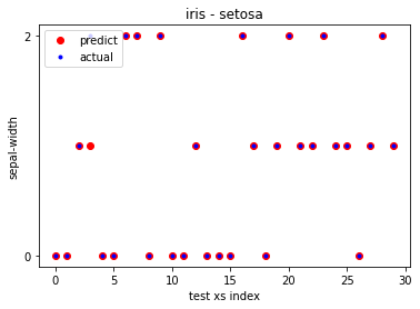
예측 결과:[0 0 1 1 0 0 2 2 0 2 0 0 1 0 0 0 2 1 0 1 2 1 1 2 1 1 0 1 2 1]
실제 결과:[0 0 1 2 0 0 2 2 0 2 0 0 1 0 0 0 2 1 0 1 2 1 1 2 1 1 0 1 2 1]
실제 값과 예측 값을 도표로 표시해 볼게요.
import matplotlib.pyplot as plt
plt.plot(pred_val,'ro',label='predict')
plt.plot(test_ys,'b.',label='actual')
plt.xlabel('test xs index')
plt.ylabel('sepal-width')
plt.yticks([0,max(max(pred_val),max(test_ys))])
plt.legend()
plt.title('iris - setosa')
plt.show()

전체 중에 한 개만 차이가 있네요. 함수를 만들어서 확인해 볼게요.
def evaluate(actual_ys, predict_ys):
  correct_cnt = 0
  for i,y in enumerate(actual_ys):
    if predict_ys[i] == actual_ys[i]: #일치하면
      correct_cnt+=1
  return correct_cnt/len(actual_ys) #맞춘 개수/ 전체 개수
함수를 호출해서 확인해 봅시다.
print(evaluate(test_ys,pred_val))
출력 결과
0.9666666666666667
3. 사이킷 런의 KNN 사용하기
사이킷 런의 KNN 중에 여기에서는 분류 모델을 사용합니다.
from sklearn.neighbors import KNeighborsClassifier
모델을 생성한 후 학습할게요.
knc_model = KNeighborsClassifier()
knc_model.fit(train_xs,train_ys) #학습
pred_val2 = knc_model.predict(test_xs) #예측
예측 결과와 실제 결과를 출력해 볼게요.
print(f'예측 결과:{pred_val2}')
print(f'실제 결과:{test_ys}')
출력 결과
예측 결과:[0 0 1 1 0 0 2 2 0 2 0 0 1 0 0 0 2 1 0 1 2 1 1 2 1 1 0 1 2 1]
실제 결과:[0 0 1 2 0 0 2 2 0 2 0 0 1 0 0 0 2 1 0 1 2 1 1 2 1 1 0 1 2 1]
예측 후에 스코어평가 스코어를 확인합시다.
print(knc_model.score(test_xs,test_ys)) #평가 스코어
출력 결과
0.9666666666666667
도표로 예측 결과와 실제 결과를 표시할게요.
plt.plot(pred_val2,'ro',label='predict')
plt.plot(test_ys,'b.',label='actual')
plt.xlabel('test xs index')
plt.ylabel('sepal-width')
plt.yticks([0,max(max(pred_val2),max(test_ys))])
plt.legend()
plt.title('iris - setosa')
plt.show()
이상으로 KNN 분류 모델이 어떠한 원리로 동작하는지 알아보았습니다.