
안녕하세요. 언제나 휴일입니다.
동영상 강의는 언제나 휴일 유튜브에서 제공하고 있어요.
정규분포는 자연 세계를 표현할 때 가장 많이 사용하는 분포 중 하나로 가우시안 분포라고도 부릅니다.
중심극한정리에서는 독립적인 확률 변수들의 평균은 정규 분포를 따른다고 증명하고 있습니다.
https://ko.wikipedia.org/wiki/%EC%A4%91%EC%8B%AC_%EA%B7%B9%ED%95%9C_%EC%A0%95%EB%A6%AC(위키백과 – 중심극한정리)
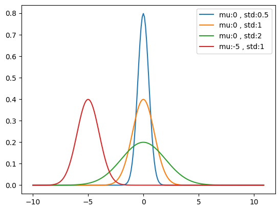
다음은 평균(mu)과 표준편차(std)에 따른 정규 분포 곡선입니다.
정규분포 관련 함수는 norm 모듈에서 제공합니다.
import scipy as sp
from scipy import stats
from scipy.stats import norm
정규 분포를 따르는 샘플 생성하기
데이터 과학에서는 정규 분포를 따르는 모집단(혹은 표본집단)의 평균과 표준편차를 알고 있다면 rvs함수를 이용하여 샘플을 만들 수 있습니다.
예를 들어, 20XX년 A시의 성인 남성의 평균 키가 174cm이고 표준 편차가 7이라고 가정할게요.
이 때 이러한 특징을 갖는 100개의 가상 샘플을 만든다면 다음처럼 norm의 rvs 함수를 이용하여 만들 수 있어요.
rvs에 size에는 샘플 수, loc에는 평균, scale에는 평균을 전달합니다.
mu = 174 #평균
std = 7 #표준편차
n = 100 #샘플 수
samples = norm.rvs(size=n,loc=mu, scale =std)
samples
[out]
array([164.71382232, 168.24642781, 171.62934239, 170.19511216,
162.70987793, 176.00179872, 171.05801384, 169.76359984,
173.36469118, 176.4193017 , 171.47178961, 168.3369376 ,
173.023286 , 184.51912098, 177.94061235, 190.96526004,
167.53268702, 168.66300393, 176.33199273, 174.11948492,
167.56943772, 189.27586309, 172.97008829, 167.89064864,
172.60147949, 164.08899082, 182.15093262, 165.73545528,
173.35146376, 168.51085353, 176.93683555, 177.9329996 ,
181.90534466, 172.01924201, 176.25655301, 174.36186104,
169.99538721, 183.18791928, 175.8714226 , 176.76429583,
162.39749033, 172.03996626, 177.31723426, 171.77266015,
171.54199017, 161.98945354, 171.07154196, 177.51824705,
176.07467692, 171.0804016 , 178.00662214, 175.74109779,
177.44499487, 173.31318938, 172.25723787, 176.93153927,
182.17699037, 182.34551537, 187.2789279 , 157.73228803,
165.35027586, 178.18712333, 170.04117188, 180.06368978,
185.01409712, 176.1707225 , 169.74742848, 174.71595246,
183.28198284, 163.67926725, 180.4033461 , 178.86578095,
172.58491819, 172.25420241, 169.93826977, 167.041646 ,
185.94620753, 172.62357987, 165.35547372, 164.4659428 ,
172.3818228 , 177.04299041, 169.22727578, 181.52221902,
173.44771661, 169.46810152, 186.99649304, 175.56942259,
171.10339066, 183.07571308, 167.50775509, 172.68276163,
175.96057408, 166.1216901 , 179.7294738 , 170.88158779,
169.4601792 , 179.25755172, 171.07129907, 186.52810336])이를 다음 모듈을 이용하여 분석하고 시각화합시다.
import matplotlib.pyplot as plt
import numpy as np
import pandas as pd
먼저 pandas의 시리즈를 이용하여 개략적인 데이터 정보를 확인해 볼게요.
sd = pd.Series(samples)
sd.describe()
[out]
count 100.000000
mean 173.971825
std 6.548271
min 157.732288
25% 169.759557
50% 172.996687
75% 177.621935
max 190.965260
dtype: float64분포를 히스토그램으로 표시하면 다음처럼 작성할 수 있어요.
min_val = int(np.min(samples))-1
max_val = int(np.max(samples))+1
bins = range(min_val,max_val+1)
plt.hist(samples,bins=bins)
plt.title(f'sample count = {n}')
plt.show()
[out]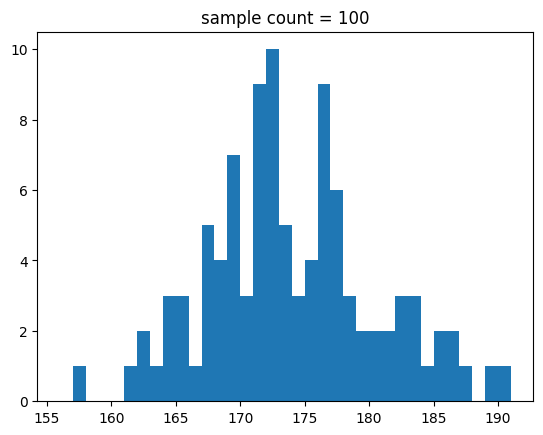
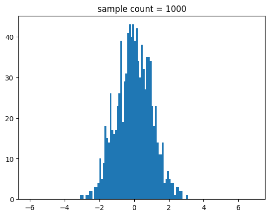
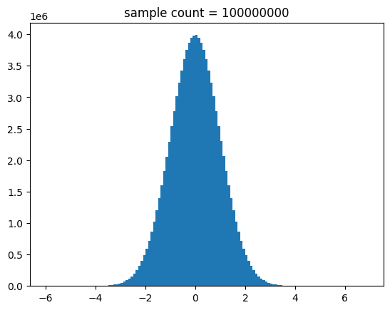
생성한 샘플에 따라 분포를 나타내 볼게요.
def show_norm_samples_hist(mu = 0,std = 1,n = 1000):
  samples = norm.rvs(size=n,loc=mu, scale =std)
  min_val = int(np.min(samples))-1
  max_val = int(np.max(samples))+1
  bins = range(min_val,max_val+1)
  plt.hist(samples,bins=bins)
  plt.title(f'sample count = {n}')
  plt.show()
import math
for i in range(2,9):
n = int(math.pow(10,i))
show_norm_samples_hist(mu=174, std=7, n=n)[out]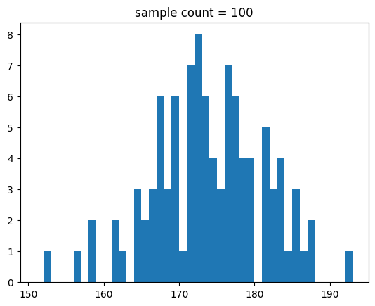
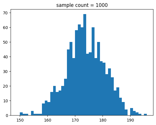
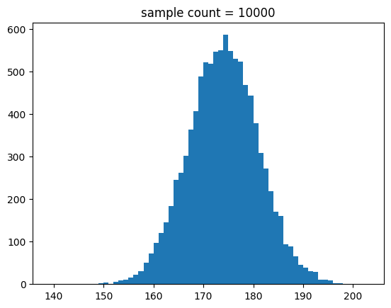
중간 출력 결과는 생략할게요.
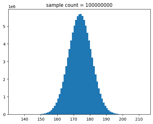
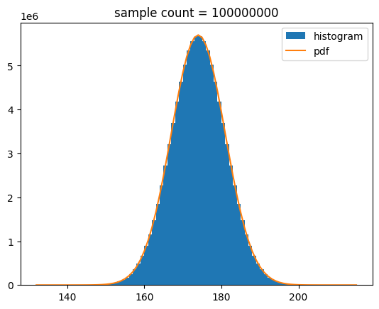
결과를 보면 알 수 있듯이 샘플 수가 많아지면 정규 분포 곡선에 유사해 짐을 알 수 있어요.
샘플의 분포를 표준 점수로 변환 후 도식화
데이터의 크기에 관계없이 비교를 하기 위해 스케일을 표준화를 합니다.
표준 점수(zscore)는 표본에 평균을 뺀 후에 표준 편차로 나누어 구할 수 있습니다.
zscore = (sample -mean)/std
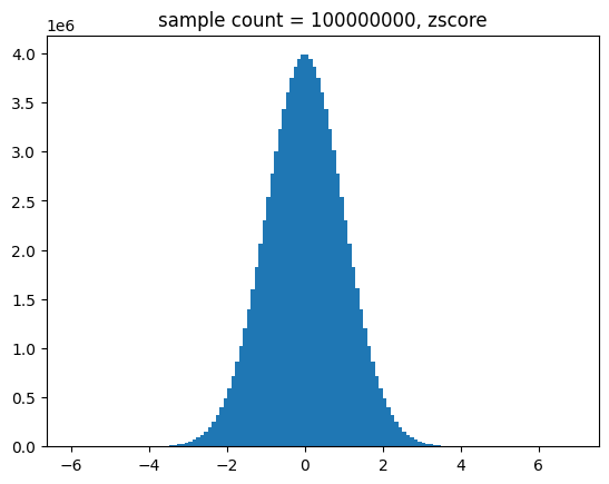
다음은 정규 분포를 따르는 샘플을 생성한 후에 표준 점수로 변환 후에 분포를 도식한 것입니다.
def show_norm_samples_z_hist(mu = 0,std = 1,n = 1000):
  samples = norm.rvs(size=n,loc=mu, scale =std)
  z_scores = (samples - mu) /std
  bins = np.arange(-6,7,0.1)
  plt.hist(z_scores,bins=bins)
  plt.title(f'sample count = {n}, zscore')
  plt.show()
import math
for i in range(2,9):
n = int(math.pow(10,i))
show_norm_samples_z_hist(mu=174,std=7,n=n)[out]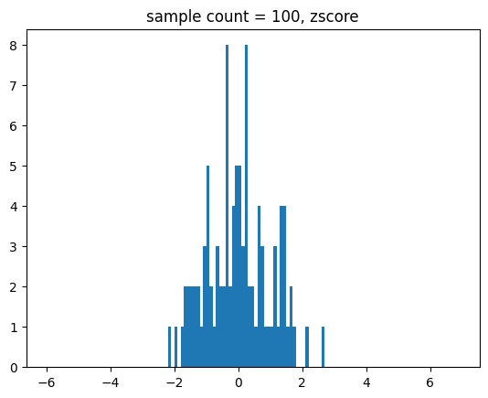
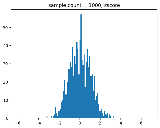
중간 출력 결과는 생략할게요.
표준 정규 분포를 따르는 샘플 생성하기
평균이 0이고 표준 편차가 1인 정규 분포를 표준 정규 분포라고 부릅니다.
이는 정규 분포를 표준 점수로 스케일을 변환하면 나오는 정규 분포입니다.
norm.rvs 함수의 평균(loc)과 표준 편차(scale) 인자의 디폴트 값은 0과 1입니다. 따라서 해당 인자를 전달하지 않으면 표준 정규 분포를 따르는 샘플을 생성합니다.
다음은 표준 편차를 따르는 100개의 샘플을 만드는 코드입니다.
samples = norm.rvs(size=100) #평균이 0이고 표준편차가 1일 정규 분포 샘플을 생성
samples
[out]
array([-2.26590825e-02, 7.68598954e-01, 1.53703335e+00, 1.03700761e+00,
1.33181844e-02, 3.51002070e-01, 7.89846360e-01, -8.53795074e-02,
1.89154536e-01, -1.69774669e-01, -8.37227730e-01, 1.02584194e+00,
1.74926191e-01, -7.90466136e-01, -6.01688111e-01, -9.46922018e-02,
2.96171880e-01, -2.57342784e-01, -1.68538710e-01, 8.38380834e-01,
-5.81038297e-01, 8.60378248e-01, 2.07922108e+00, 8.34765785e-01,
1.90486951e+00, 9.26192353e-01, 9.00123284e-01, -2.55537387e-01,
-2.34421471e-03, 6.31187820e-01, -7.54889103e-01, 3.35330364e-01,
2.23957352e-01, -1.05408630e+00, 2.72312891e-01, -1.58867535e+00,
1.07963275e+00, -2.21600340e+00, -7.42057386e-02, -1.33913751e+00,
1.15480647e+00, -3.60585574e-01, 3.00159496e-01, -3.17080364e-01,
1.70458492e+00, 1.05685668e+00, 3.66381971e-01, 2.18052666e+00,
-2.42398715e-02, 2.06202745e-01, -1.02456799e+00, -1.06020147e+00,
8.72137038e-01, 2.15144183e-01, 4.16632859e-01, -8.04096072e-01,
1.69091449e+00, -4.71019906e-02, 1.62583171e-01, 2.31805510e+00,
-5.03251934e-01, 1.16465879e+00, 5.07379685e-01, 1.43181687e+00,
2.68522436e-02, 8.60729245e-01, 3.07096746e-02, -9.58554717e-01,
-1.50783058e+00, 1.14388400e+00, -1.43754750e+00, 6.72227997e-01,
-1.71676076e+00, 7.80825103e-01, -1.08592331e+00, 6.70279357e-01,
-7.17350865e-01, 1.32926529e+00, 6.88717753e-01, 4.53680089e-01,
-4.68894704e-01, -7.38673322e-01, 2.03618906e+00, -3.75616109e-01,
-2.67825738e-01, -7.20943659e-01, 7.47110164e-01, 2.19722144e-01,
5.86028904e-01, -7.97794208e-01, 1.94837165e+00, -1.47164904e+00,
-5.38386276e-01, 8.65327780e-01, 1.27140813e+00, 1.08613668e+00,
-1.12173149e+00, 2.41422069e+00, 1.30174752e+00, 6.07858846e-01])pandas의 시리즈로 데이터 기초 정보를 확인해 볼게요.
sd = pd.Series(samples)
sd.describe()
[out]
count 1.000000e+08
mean 1.543317e-04
std 1.000114e+00
min -5.739074e+00
25% -6.744843e-01
50% 2.090137e-04
75% 6.747330e-01
max 5.988447e+00
dtype: float64다음은 표준 정규 분포를 따르는 샘플을 생성한 후에 분포를 도식화하는 코드입니다.
def show_stdnorm_samples_hist(n = 1000):
  samples = norm.rvs(size=n)
  bins = np.arange(-6,7,0.1)
  plt.hist( samples  ,bins=bins)
  plt.title(f'sample count = {n}')
  plt.show()
[out]
for i in range(2,9):
n = int(math.pow(10,i))
show_stdnorm_samples_hist(n=n)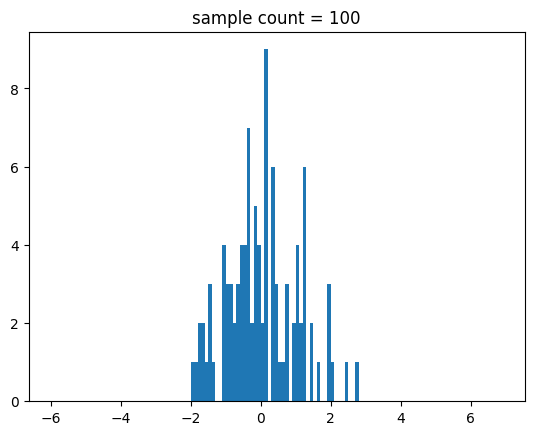
중간 출력 결과를 생략할게요.
확률 밀도 함수
확률 변수의 분포를 나타내기 위해 확률 밀도 함수를 제공합니다.
이는 확률 변수 X가 구간 [a,b]에 포함될 확률을 구하는 함수입니다.
help(norm.pdf)[out]
Help on method pdf in module scipy.stats._distn_infrastructure:
pdf(x, *args, **kwds) method of scipy.stats._continuous_distns.norm_gen instance
Probability density function at x of the given RV.
Parameters
----------
x : array_like
quantiles
arg1, arg2, arg3,... : array_like
The shape parameter(s) for the distribution (see docstring of the
instance object for more information)
loc : array_like, optional
location parameter (default=0)
scale : array_like, optional
scale parameter (default=1)
Returns
-------
pdf : ndarray
Probability density function evaluated at x앞에서 작성한 정규 분포를 따르는 샘플과 확률 밀도 함수를 표본 개수에 맞게 보정하여 함께 그려보기로 할게요.
def show_norm_samples_pdf(mu = 0,std = 1,n = 1000):
  samples = norm.rvs(size=n,loc=mu, scale =std)
  min_val = int(np.min(samples))-1
  max_val = int(np.max(samples))+1
  bins = range(min_val,max_val+1)
  y = norm.pdf(bins,mu,std)*n
  plt.hist(samples,bins=bins,label='histogram')
  plt.plot(bins,y,label='pdf')
  plt.legend()
  plt.title(f'sample count = {n}')
  plt.show()
import math
for i in range(2,9):
n = int(math.pow(10,i))
show_norm_samples_pdf(mu=174,std=7,n=n)[out]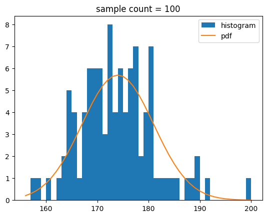
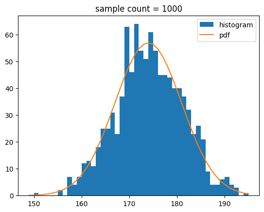
중간 출력 결과는 생략할게요.
누적 밀도 함수
확률 밀도 함수의 값을 누적한 함수로 누적 밀도 함수를 제공합니다.
확률 변수가 특정 값보다 작거나 같을 확률 등을 구할 때 사용합니다.
help(norm.cdf)[out]
Help on method cdf in module scipy.stats._distn_infrastructure:
cdf(x, *args, **kwds) method of scipy.stats._continuous_distns.norm_gen instance
Cumulative distribution function of the given RV.
Parameters
----------
x : array_like
quantiles
arg1, arg2, arg3,... : array_like
The shape parameter(s) for the distribution (see docstring of the
instance object for more information)
loc : array_like, optional
location parameter (default=0)
scale : array_like, optional
scale parameter (default=1)
Returns
-------
cdf : ndarray
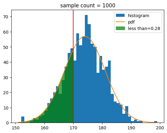
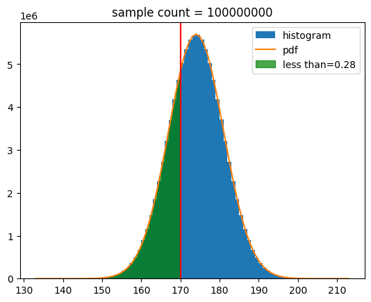
Cumulative distribution function evaluated at `x`평균 키가 174cm이고 표준 편차가 7일 때 170cm 이하일 확률은 x값에 170을 전달하여 쉽게 구할 수 있어요.
norm.cdf(loc=174,scale=7,x=170)[out]
0.2838545830986763정규 분포를 따르는 샘플과 누적 확률 밀도 함수를 같이 그려 봅시다.
def show_norm_samples_cdf(mu = 0,std = 1,n = 1000, value=mu):
  samples = norm.rvs(size=n,loc=mu, scale =std)
  min_val = int(np.min(samples))-1
  max_val = int(np.max(samples))+1
  bins = range(min_val,max_val+1)
  py = norm.pdf(bins,mu,std)*n
  cy = norm.cdf(loc=mu,scale=std,x=value)
  plt.hist(samples,bins=bins,label='histogram')
  plt.plot(bins,py,label='pdf')

  bins2 =  range(min_val,int(value)+1)
  py2 = norm.pdf(bins2,mu,std)*n
  plt.fill_between(bins2,py2,alpha=0.7,color='green',label=f'less than={cy:.2f}')

  plt.axvline(value,color='r')
  plt.legend()
  plt.title(f'sample count = {n}')
  plt.show()
import math
for i in range(2,9):
n = int(math.pow(10,i))
show_norm_samples_cdf(mu=174,std=7,n=n,value=170)[out]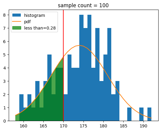
생존확률
생존 확률은 1-cdf입니다.
help(norm.cdf)[out]
Help on method cdf in module scipy.stats._distn_infrastructure:
cdf(x, *args, **kwds) method of scipy.stats._continuous_distns.norm_gen instance
Cumulative distribution function of the given RV.
Parameters
----------
x : array_like
quantiles
arg1, arg2, arg3,... : array_like
The shape parameter(s) for the distribution (see docstring of the
instance object for more information)
loc : array_like, optional
location parameter (default=0)
scale : array_like, optional
scale parameter (default=1)
Returns
-------
cdf : ndarray
Cumulative distribution function evaluated at `x`
평균 키가 174cm이고 표준 편차가 7일 때 170cm 이하일 확률과 170cm 초과일 확률을 구한다면 다음처럼 cdf 함수를 호출하여 구할 수 있어요.
a =  norm.cdf(loc=174,scale=7,x=170)
b = 1 -a
print(f"170 이하일 확률:{a:.2f}")
print(f"170 초과일 확률:{b:.2f}")
[out]
170 이하일 확률:0.28
170 초과일 확률:0.72170 초과일 때 sf 함수를 호출하여 구할 수도 있습니다.
a =  norm.cdf(loc=174,scale=7,x=170)
b = norm.sf(loc=174,scale=7,x=170)
print(f"170 이하일 확률:{a:.2f}")
print(f"170 초과일 확률:{b:.2f}")
[out]
170 이하일 확률:0.28
170 초과일 확률:0.72퍼센트 포인트 함수
누적 확률이 특정 퍼센트일 때의 값을 구하는 함수입니다.
help(norm.ppf)[out]
Help on method ppf in module scipy.stats._distn_infrastructure:
ppf(q, *args, **kwds) method of scipy.stats._continuous_distns.norm_gen instance
Percent point function (inverse of `cdf`) at q of the given RV.
Parameters
----------
q : array_like
lower tail probability
arg1, arg2, arg3,... : array_like
The shape parameter(s) for the distribution (see docstring of the
instance object for more information)
loc : array_like, optional
location parameter (default=0)
scale : array_like, optional
scale parameter (default=1)
Returns
-------
x : array_like
quantile corresponding to the lower tail probability q.평균 키가 174cm이고 표준 편차가 7일 때 상위 30%인 키를 구한다면 ppf함수를 호출하세요.
norm.ppf(loc=174,scale=7,q=0.7)[out]
177.6708035889563